< H X A 7 2 4 1 > : MiniLight minimal global illumination renderer

description

MiniLight is a minimal global illumination renderer. It is primarily an exercise in simplicity. But that makes it a good base and benchmark (in some sense) for development and experimentation. And it just might be the neatest renderer around (on average, about 650 lines). There are translations into several programming languages.

Someone asked me how to develop a renderer in three months. It seemed not nearly enough time. But then I began to think how small such a program could be, whilst still being a complete physically based simulation with a clear, well-formed design. (A somewhat different aim from the ‘Minimal Ray Tracer Programming Contest’ of 1987.) I couldn't resist an attempt.

It is a command-line application. It reads a simple text model file and writes a PPM image file. Supported platforms include Mac , Linux , and Windows .

The rendering features are:

Monte-carlo path-tracing transport
Emitter sampling
Progressive refinement
RGB light
Diffuse materials
Triangle modelling primitives
Octree spatial index
Pin-hole ‘lens’
Ward linear tone-mapping

Full source code is provided under the (new) BSD license or UNLICENSE.

images

A Cornell Box (of course) throughout the day:

Cornell Box, at morning (24 KB)

Cornell Box, at noon (23 KB)

Cornell Box, at evening (26 KB)

Cornell Box, at night (23 KB)

The models are physically based too. For example, at noon: The sky has a colour temperature of 10000K and a luminance of 1 x 10⁴ cd/m². The sun has a colour temperature of 5400K and a luminance of 1 x 10⁹ cd/m², a diameter of 1.392 x 10⁹ m, and distance of 149.6 x 10⁹ m. (It is just a square though.)

Some of the Smits test scenes:

Smits tests (32 KB)

A room, at noon-ish, and night (made in HDR and tonemapped with p3tonemapper):

Front room, at noon (97 KB)

Front room, at night (47 KB)

All these renders are 1000 paths per pixel. The standard Cornell Box, at 500 x 500 pixels, should take about 15 minutes on a 2007 machine.

comparison

There are now nine+ translations:

language (and version)	size (lines of code)	size (relative to C++)	speed (relative to C++)
Scala 2.7.7	431	0.45	1 / 2.7
OCaml 3.11.0	457	0.48	1 / 2.3
Python 2.5.1	490	0.52	1 / 180
Python Shed Skin 0.1.1	496	0.52	1 / 1.8
Ruby 1.8.6	498	0.52	1 / 218
Lua 5.1.4	568	0.60	1 / 52
LuaJIT 2.0.0 beta 3	568	0.60	1 / 13
C# 3.5	630	0.66	1 / (1–5 ?)
Flex 2/AS3 (Flash 10,0,22,87)	644	0.68	1 / 55
Scheme R5RS (Bigloo 3.6a)	665	0.70	1 / 60
C++ ISO-98 (LLVM-G++-4.2)	952	1.00	1
C ISO-90 (LLVM-GCC-4.2)	1197	1.26	2.1

Line counts disclude comments and blanks and lines with only single braces/parentheses. Flex/ActionScript3 is 864 lines including extra UI.

Speed measurements were done on a Core2-Duo Mac, using the cornellbox and roomfront (non-sun) models. They will vary with platform and model.

C was much faster than C++ because LLVM's link-time optimisation worked for C, but not for C++ (otherwise, C would likely be about 10% faster).

Scala, Lua, Ruby and Flex are twice as slow without some manual optimization (Python too, probably). This is mostly inlining some vector operations (but also a little loop unrolling, and flattening the image pixel array).

Try the Flex version here . . .

algorithm

path tracing

The simplest method of global illumination is pure monte-carlo path tracing. For each pixel, a ray is sent into the scene. When it hits something it notes its color and emission. It then bounces off and continues. Eventually all the noted info is sent back, step by step. Each step scales the light by certain factors until a final value is returned to the pixel. Repeat the whole process many times with some randomness added and average all the results. An image slowly emerges.

This strategy is essentially a blind search for light emitters. Unless a ray hits an emitter it will return only blackness. For outdoor scenes most rays will bounce into the sky, and find brightness. But for indoors the emitters are small and many many rays are needed to find them. It is too slow.

emitter sampling

This can be alleviated with emitter sampling. The location of all emitters is known from the model, and this can be used. Each step sends an extra ray to an emitter. But now there are two rays gathering the incoming light they must not duplicate any. To ensure this, ‘local’ emission at each bounce is no longer included.

monte carlo

Each interaction along the main path is handled mostly by monte-carlo. The bounce direction is chosen by importance sampling: proportionally more likely in directions the surface allows more reflection through. For ideal diffuse that is lots near perpendicular, little near grazing. The overall reflectivity is controlled by russian-roulette: proportionally more likely to bounce the more reflective the surface is. This allows a non-arbitrary end for the recursion. The colour is just scaling, because there is no advantage in monte-carlo there.

Both uses of monte-carlo sample more where the surface interaction transfers more light. This is a fairly good approach.

Why? A simple analysis is that apparent noisiness is the product of detail/richness and intensity: greater detail means adjacent pixels more likely see different values, greater intensity probably means more contrast. The latter is easiest to address, because interaction's effect on intensity is simple. The treatment—sampling more—reduces noise by averaging-out the effect of the randomness.

Over many iterations this puts more computation into resolving more visibly noisy regions, rather than wasting it on regions that won't noticeably improve. That computes an image of particular quality more quickly. But there are still shortcomings . . .

rendering equation

Here is the specific rendering equation for this algorithm:

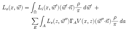
$L_o(x, \vec w) = \int_\Omega L_i(x, \vec w') (\vec w' \cdot \vec n) \frac{\rho}{\pi}\, d\vec w' \ \ + \ \ \sum_E\int_A L_e(z, \vec w'') \Gamma_A V(x,z) (\vec w'' \cdot \vec n) \frac{\rho}{\pi}\, d a$

Meaning: The radiance outward at a position and direction equals the sum of two terms (the first representing the main path, the second the emitter sampling). The first term integrates over the surrounding hemisphere of directions the inward radiance scaled by its projection and the reflectivity function. The second term sums over all emitters, for each integrating over the area the emission scaled by the solid angle, the visibility, the projection, and the reflectivity function.

unbiased?

Monte-carlo path-tracing is described as ‘unbiased’. The term is now sometimes used in the manner of a marketing tag. Its real meaning is too abstract for that purpose. It denotes a lack of consistent error—the only error is in the effects of the randomness. Such niceties are appropriate for mathematics but for engineering we must live by practicalities. All implementations are biased and incorrect in various ways. The task is to arrange them acceptably.

ultimately

The value of this method is its simplicity, while having full generality. It allows the implementation to be almost proven correct by inspection. (Correct meaning ‘following the rules for a particular standard approximation’.) The images produced can be authoritative references for other renderers.

The core idea has also proven remarkably durable and adaptable since Whitted's paper of 1980. One could reasonably call it the key engineering concept for rendering, and it looks to remain so.

pseudocode

Here is the algorithmic structure in high-level pseudocode/PDL (produced by editing the code comments into a reduced form).

Whereas the actual source-code is broken into modules and procedures, this represents the sequence in a single coherent view. Thought of like geographic maps, the first is roughly 38:1 scale, the second 10:1.

High-level – 38:1 Scale

17 lines – roughly 1 for every 38 of actual code.

- render, by progressive refinement
   - render a frame, to the image
      - sample each image pixel
         - make sample ray direction
         - get radiance returning in sample direction
            - intersect ray with scene
            - if intersection hit
               - get local emission (only for first-hit)
               - calculate emitter sample
               - calculate recursive reflection
               - sum local emission, emitter sample, and recursive reflection
            - else no hit
               - use default/background scene emission
         - add radiance to image
   - save image
      - divide pixel values by frame count
      - apply tonemapping factor

Medium-level – 10:1 Scale

66 lines – roughly 1 for every 10 lines of actual code.

- render, by progressive refinement, as many frames as wanted
   - render a frame, to the image
      - sample each image pixel
         - make sample ray direction (with sub-pixel jitter)
         - get radiance returning in sample direction

            - intersect ray with scene
               - if octree branch
                  - step through subcells and recurse
                    - find which subcell holds ray origin
                    - step through intersected subcells
                       - intersect nested subcell (by recursing)
                       - exit branch if triangle hit
                       - find next subcell ray moves to
                       - move to (outer face of) next subcell, or exit branch
               - else octree leaf
                  - exhaustively intersect contained triangles
                     - avoid false intersection with triangle just come from
                        - intersect ray with triangle
                           - check if nearest so far
                              - check intersection is inside cell bound
                                 - note hit details

            - if intersection hit
               - get local emission (only for first-hit)
                  - read triangle attribute

               - calculate emitter sample:
                 emissive area, ideal diffuse BRDF:
                    reflected = (emitivity * solidangle) * (emitterscount) *
                       (cos(emitdirection) / pi * reflectivity)
                  - request emitter sample point from scene
                  - if emitter sample point available
                     - if shadow ray is unshadowed
                        - calculate inward emission value
                           - emit from front face of triangle only
                              - estimate solid angle
                              - multiply emitivity by solid angle
                        - calculate amount reflected by triangle
                           - check both directions are on same side of triangle
                             (no transmission)
                              - calculate ideal diffuse BRDF:
                                radiance scaled by reflectivity, cos, and 1/pi
                        - scale radiance by number of emitters in scene

               - calculate recursive reflection:
                 single hemisphere sample, ideal diffuse BRDF:
                    reflected = (inradiance * pi) * (cos(in) / pi * color) *
                       reflectance
                 reflectance magnitude is 'scaled' by the russian roulette,
                 cos is importance sampled, and the pi and 1/pi cancel out,
                 leaving just: inradiance * reflectance color
                  - calculate next direction
                     - do russian-roulette with reflectivity 'magnitude'
                     - if alive
                        - make direction as cosine-weighted importance sample of
                          hemisphere
                        - make color by dividing-out mean from reflectivity
                  - if not path end
                     - recurse to 'get radiance returning in sample direction'
                     - scale recursed radiance by color

               - sum local emission, emitter sample, and recursive reflection

            - else no hit
               - use default/background scene emission

         - add radiance to image
   - save image periodically
      - divide pixel values by frame count
      - apply (Ward linear) tonemapping factor
      - write image file (PPM P6 format)
   - display UI feedback

downloads

Version 1.5.3 and 1.5.2
(Scheme, C, and C++ 1.5.3 updated 2011-02-08)
(Scala, Ocaml 1.5.2.1 updated 2010-01-09, 2009-04-01)
(others 1.5.2 updated 2008-02-17)

minilight153c.zip	C ISO-90 source code and Mac, Linux, and Windows executables (141 KB)
minilight153scheme.zip	Scheme R5RS source code (45 KB)
minilight15scala.zip	Scala 2.7 source code (32 KB)
minilight153cpp.zip	C++ ISO-98 source code (56 KB)
minilight15ocaml.zip	OCaml 3.11 source code (30 KB)
minilight15lua.zip	Lua 5.1 source code (28 KB)
minilight15python.zip	Python 2.5 source code (18 KB) (Translation by Juraj Sukop)
minilight15ruby.zip	Ruby 1.8 source code (25 KB)
minilight15flex.zip	Flex 2 source code (44 KB)

external

MiniLight OCaml	adjusted and varied by Mauricio Fernández
MiniLight Java	translated by Tom Eklöf
MiniLight F#	translated by Ian Voyce
MiniLight C# 3.5	translated (with small extras) by Chris Lomont
MiniLight Clojure 2009	in progress, by Mark Reid

contribution

If you can't resist doing a translation, I can probably add/link to it. It is a good way to learn 80% of a new language.

The original guidelines were a bit unusual, but anyone else is, of course, free to diverge from them:

Make it compact and simple (these are the priority), by good use of the language.
Only optimize where really needed, and not excessively (you want to find out how well the compiler/language can do for itself with no manual help).
Perhaps follow the main module separation design.
Write the best code possible!

Sacrifice some clarity for compactness in the SpatialIndex module. It is a bit large (it deserves careful testing, too). And, only to make the sizes comparable:

lines should be <= 80 chars
indent ought to be 3-ish chars (but mixing tabs and spaces is instant disqualification!)

The reference versions are the Scheme and the C.

hxa7241+www (ατ) googlem‌ail (dοτ) com

MINILIGHT